Getting started
In the following we will set up a Jupyter notebook to collect and plot data from a dummy instrument to understand the basic usage of qcodes++. No measurement hardware is required.
Setup
Assuming you installed qcodes++ as described in the installation instructions, you can start Jupyter lab from the Anaconda prompt or command line by activating the environment:
conda activate qcodespp
and starting Jupyter lab:
jupyter lab
This will open a Jupyter lab window in your browser. In the Jupyter lab, create a new Python 3 notebook and run
import qcodespp as qc
from qcodespp.instrument_drivers.instrument_mocks import DummyMeasurementInstrument
This code imports the top level of the qcodes++ package, and the DummyMeasurementInstrument driver. In general the instrument drivers are python classes which can be used to create a specific connection with a specific instrument. In this case, we ‘connect’ to our Instrument by running:
instrument = DummyMeasurementInstrument(name='instrument')
As discussed in the background section, qcodes has a virtual Station which contains all the Instrument s and Parameter s. We can initialise the Station and add our `Instrument to it by running:
station = qc.Station(add_variables=globals())
This command creates a Station object and checks all the python variables defined in the notebook. If the variable is a qcodes Instrument or Parameter, it is added to the Station.
We should also tell qcodes++ where to save the data. This is done by running:
qc.set_data_folder('data')
Getting and setting parameters
The dummy instrument has two outputs for providing voltages, and two inputs for measuring voltages from the imaginary device. You can set the output by putting a number in brackets, e.g.
instrument.output1(1.2)
or
instrument.output2(5.9)
and read the value it is set to by leaving the brackets empty, e.g.
instrument.output1()
or
instrument.output2()
To read the input values, again use empty brackets, e.g.
instrument.input1()
or
instrument.input2()
Running a measurement
So far no data has been collected; we’ve just communicated with the instrument. To collect data, we need to create a Loop, which defines the independent parameter(s) that we want to vary. In this case, we will vary the output1 parameter from 0 to 10 volts in steps of 0.1 volt, and measure both the input1 and input2 parameters at each step. For a simple 1D measurement like this, we can use:
loop = qc.loop1d(sweep_parameter=instrument.output1,
                start=0,stop=10,num=101,delay=0.1,
                device_info='dummy', instrument_info='ACdiv=1e5 DCdiv=1e3 freq=123 Hz',
                measure=[instrument.input1, instrument.input2])
Here, we have created the object loop. Inside of it, is a DataSetPP object (accessed via loop.data_set), which will hold the measurements. The details of the DataSetPP are printed. You will see the data will be saved in the ‘data’ folder we specified earlier, and the name of the data includes a counter with a unique number as well as the date and time of the measurement. The rest of the name is generated from the independent parameter settings and the text provided in device_info and instrument_info.
To run the measurement, we can invoke the run() method of the loop object, and give it a list of parameters to plot:
data=loop.run([instrument.input1, instrument.input2])
A live plot window will be opened, showing measurements of the two parameters. The run() method returns the DataSetPP object, which can also be reloaded later.
That really is how easy it is to collect data with qcodes++!
Two dimensions
If you need to loop over two independent parameters, you can use the loop2D function. For example, if we want to vary both output1 and output2, we can do:
loop=qc.loop2d(sweep_parameter=instrument.output1,
                start=0,stop=10,num=11,delay=0.1,
                step_parameter=instrument.output2,
                step_start=0,step_stop=10,step_num=11,step_delay=0.1,
                device_info='dummy',
                instrument_info='ACdiv=1e5 DCdiv=1e3 freq=123 Hz',
                measure=[instrument.input1, instrument.input2])
This function ‘steps’ instrument.output2, and at every step, it sweeps instrument.output1, and at each point on that sweep, the parameters in measure are measured.
Again, we are given information about the DataSetPP, which shows the array shapes are now indeed two dimensional.
Running the measurement is again just
loop.run([instrument.input1, instrument.input2])
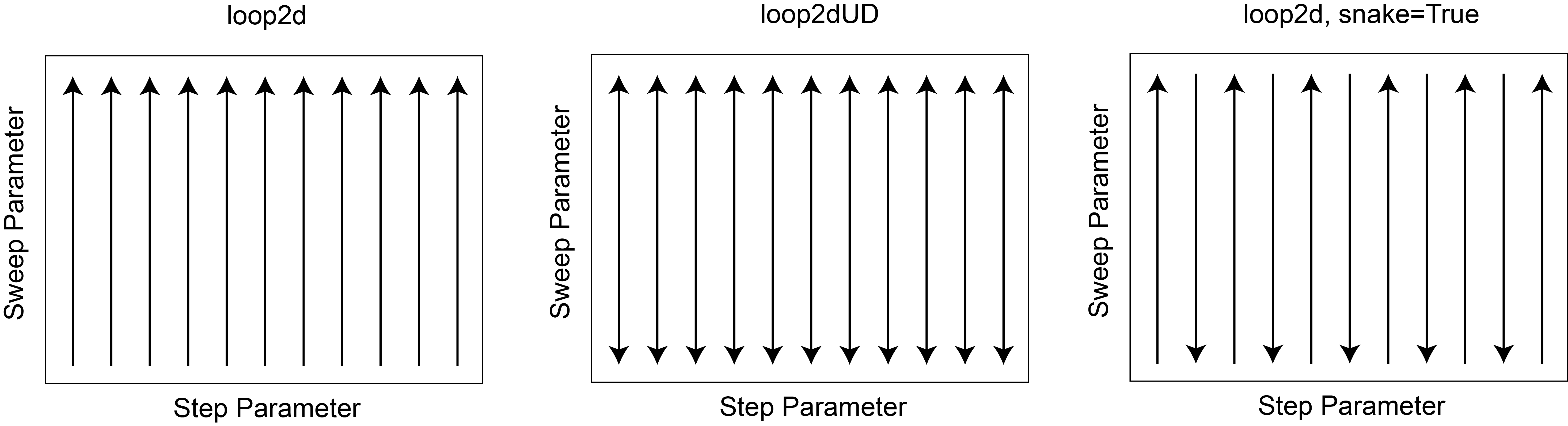
Note that in a loop2d, the sweep_parameter jumps from the stop value back to the start value every time the step_parameter is incremented. This may not be desired behaviour if your sweep_parameter is a sensitive object, e.g. a gate on a nanoelectronic device. In this case, you have two options. Firstly, you can use the loop2dUD function, where for each increment of the step_parameter, the sweep_parameter sweeps from start to stop, then from stop to start again. The code is otherwise identical.
loop=qc.loop2dUD(sweep_parameter=instrument.output1,
                start=0,stop=10,num=11,delay=0.1,
                step_parameter=instrument.output2,
                step_start=0,step_stop=10,step_num=11,step_delay=0.1,
                device_info='dummy',
                instrument_info='ACdiv=1e5 DCdiv=1e3 freq=123 Hz',
                measure=[instrument.input1, instrument.input2])
You will now see that the dataset contains two lots of data for each parameter, representing the two directions of the sweep parameter’s journey.
The other option you have is to turn on the snake behaviour in loop2d. This alters the direction of the sweep_parameter every alternate step of the step_parameter. This is done by setting the snake attribute to True:
loop=qc.loop2d(sweep_parameter=instrument.output1,
                start=0,stop=10,num=11,delay=0.1,
                step_parameter=instrument.output2,
                step_start=0,step_stop=10,step_num=11,step_delay=0.1,
                device_info='dummy',
                instrument_info='ACdiv=1e5 DCdiv=1e3 freq=123 Hz',
                snake=True,
                measure=[instrument.input1, instrument.input2])
Here is a visualisation of the three types of 2D loops:
The loop2dUD function has the option to sweep the sweep_parameter with a fewer number of increments on the return sweep. To set this scaling factor, provide an integer to the fast_down attribute. For example, if you want to sweep the sweep_parameter with 101 increments on the up-sweep, and only 20 increments on the down-sweep, you can do:
loop=qc.loop2dUD(sweep_parameter=instrument.output1,
                start=0,stop=10,num=101,delay=0.1,
                step_parameter=instrument.output2,
                step_start=0,step_stop=10,step_num=11,step_delay=0.1,
                device_info='dummy',
                instrument_info='ACdiv=1e5 DCdiv=1e3 freq=123 Hz',
                fast_down=5,
                measure=[instrument.input1, instrument.input2])
Other sweep types
By default the above loop functions sweep and step linearly. You can use a logarithmic scaling by specifying sweep_type='log' or step_type='log', which uses numpy’s geomspace. You can also use sweep_type='return' or step_type='return', which returns to the start value after reaching the stop value. See the Sweep types section for more information.
Higher dimensions
If you have three or more independent parameters, you will need to manually construct your loop, by explicitly using the Loop class, and/or with the help of python loops.
No dimensions: Measure class
If you don’t need a loop at all, e.g. you simply need to save data from an instrument’s buffer to disk, you can use the Measure class. See the Measure class section for more information.